A Comprehensive Guide to Auto-Encoders in Neural Networks"
In our last section we have seen what is ResNet and how to implement it. In this article we will look at AutoEncoders and how to implement it in PyTorch.
Introduction
Auto-encoders are a type of nepytorch autoencoder tutorial,ural network that have gained popularity in recent years due to their ability to learn efficient representations of data. They are used in a variety of applications such as image and speech recognition, and anomaly detection.
What are AutoEncoder ?
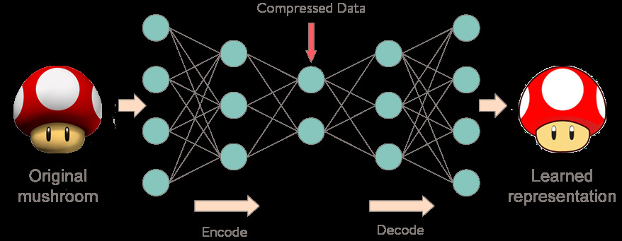
Well according to wikipedia “It is an artificial neural network used to learn efficient data encoding”. Basically autoencoder compreses the data or tu put it in other word it transform the data of heigher dimenssion to lower dimenssion by learninh how to ignore noises. The encoder part in an autoencoder learns how to compress the data into lower domenssion, while the decoder part learns how to reconstruct original data from the encoded data.
Autoencoder are used in deepfake where the idea is we train two autoencoder both on different kind of datasets and then we use first autoencoder’s encoder to encode the image and second autoencoder’s decoder to decode the encoded image.
Here is an example of deepfake.

Beside this autoencoder are also used in GAN-Network for generating image,image compression,image dignosing etc.
How do Auto-Encoders Work?
Auto-encoders work by learning a compressed representation of the input data that captures its essential features. This compressed representation can be used for tasks such as data visualization, feature extraction, and anomaly detection.
The training of an auto-encoder involves minimizing a loss function that measures the difference between the input and the reconstructed output. The most common loss function used for auto-encoders is the mean squared error (MSE) loss.
Applications of Auto-Encoders
Auto-encoders have a wide range of applications in various fields. They are used for image and speech recognition, natural language processing, and anomaly detection.
In image and speech recognition, auto-encoders are used to learn compact representations of images and audio signals that can be used for classification and other tasks. In natural language processing, auto-encoders are used to learn representations of words and sentences that can be used for tasks such as sentiment analysis and machine translation.
AutoEncoder Components
- Encoder:
Here the model learn how to compress or reduce the input dimenssions of the input data to the encoded representation or lower representation.
- Decode:
Here the model learn how to reconstruct the encoded representaion to it’s original form or close to it’s original form.
- Bottleneck:
It is the compressed representation of the input data. This is the lowest possible dimenssion of the input data.
- Reconstruction Loss:
This is the method which tell us how well the decoder perfromed in reconstructing data and how close the ouput is to the original data
Architecture of AutoEncoder
The network architecture for autoencoders can vary between a simple FeedForward network, LSTM network or Convolutional Neural Network depending on the use case.
Implementation AutoEncoder

Let’s now implement a basic autoencoder. For the dataset we will be using STL10. First let’s import necessary modules. Create a new file name main.py and write the following code :
#main.py

#! /usr/bin/env python
import torch
import numpy as np
import torchvision
import torch.nn as nn
from tqdm import tqdm
from AutoEncoder import AutoEncoder ## Our AutoEncoder Model
import matplotlib.pyplot as plt
import torchvision.transforms as transforms
from torchvision.utils import save_image

__DEBUG__ = True
LOAD = True
PATH = "./autoencoder.pth"

DEVICE = torch.device("cuda:0" if torch.cuda.is_available() else "cpu")

TRANSFORM = transforms.Compose([transforms.Resize((32,32)),transforms.ToTensor(),
                    transforms.Normalize((0.5,0.5,0.5),(0.5,0.5,0.5))])

EPOCHS = 50
BATCH_SIZE = 4
Downloading and transforming dataset
#main.py

def get_dataset(train = True):
    trainset = torchvision.datasets.STL10(root = '../dataset',
                            download = True,transform= TRANSFORM)
    trainLoader = torch.utils.data.DataLoader(trainset,batch_size = BATCH_SIZE,
                                        shuffle = True,num_workers = 8)
    return trainLoader

def imshow(img):
    img = img / 2 + 0.5     # unnormalize
    npimg = img.numpy()
    plt.imshow(np.transpose(npimg, (1, 2, 0)))
    plt.show()

def showRandomImaged(train):
    # get some random training images
    dataiter = iter(train)
    images, labels = dataiter.next()

    # show images
    print(images.shape)
    imshow(torchvision.utils.make_grid(images))
The get_dataset method will download and tranform our data for our model. It take one argument train is set to true it will give us trainning dataset and if it is false it will give us testing dataset. This method return an DataLoader object which is used in trainning.
Now let’s write our AutoEncoder. Open new file name AutoEncoder.py and write the following code:
AutoEncoder
#AutoEncoder.py

# Encoder
class Encoder(nn.Module):

    def __init__(self): super(Encoder,self).__init__()

        self.layer1 = nn.Sequential(
        nn.Conv2d(3, 16, kernel_size=5,stride = 1, padding = 2),
        nn.ReLU(),
        nn.BatchNorm2d(16),
        nn.Conv2d(16,32,kernel_size = 5, stride = 1, padding = 2),
        nn.ReLU(),
        nn.BatchNorm2d(32))

        self.layer2 = nn.Sequential(
        nn.Conv2d(32, 64, kernel_size=5,stride = 1, padding = 2),
        nn.ReLU(),
        nn.BatchNorm2d(64),
        nn.Conv2d(64,128,kernel_size = 5, stride = 1, padding = 2),
        nn.ReLU())

        self.fc1 = nn.Linear(32*32*128,1000)
        self.fc2 = nn.Linear(1000,100)


    def forward(self,x):
        x = self.layer1(x)
        x = self.layer2(x)
        x = x.view(x.size(0),-1)
        x = self.fc1(x)
        x = self.fc2(x)
        return x
In my previous article I have explained why we import nn.Module and use super method. Now let jump to our layer1 which consists of two conv2d layers followed by ReLU activation function and BatchNormalization. self.layer1 takes 3 channel as input and gives out 32 channel as output.
Similarly self.layer2 takes 32 channel as input and give out 128 channel as ouput.
Note: Here dimenssion of image is not being changed
Next we create two fully connected layer layers self.fc1 and self.fc2.
In forward method we define who our data is followed first we pass the data to layer1 followed by layer2. After that we flatten our 2D data to 1D vector using x.view method. Now our data is ready to pass through fully connected layer fc1 and fc2
Now let’s write our Decoder:
class Decoder(nn.Module):
    def __init__(self):
        super(Decoder,self).__init__()
        self.fc1 = nn.Linear(100,1000)
        self.fc2 = nn.Linear(1000,32*32*128)

        self.layer1 = nn.Sequential(
        nn.ConvTranspose2d(128, 64, kernel_size=5,stride = 1, padding = 2),
        nn.ReLU(),
        nn.BatchNorm2d(64),
        nn.ConvTranspose2d(64,32,kernel_size = 5, stride = 1, padding = 2),
        nn.ReLU(),
        nn.BatchNorm2d(32))

        self.layer2 = nn.Sequential(
        nn.ConvTranspose2d(32,16, kernel_size=5,stride = 1, padding = 2),
        nn.ReLU(),
        nn.BatchNorm2d(16),
        nn.ConvTranspose2d(16,3,kernel_size = 5, stride = 1, padding = 2),
        nn.ReLU())


    def forward(self,x):
        x = self.fc1(x)
        x = self.fc2(x)
        x = x.view(x.size(0), 128, 32, 32)
        x = self.layer1(x)
        x = self.layer2(x)

        return x
As you can clearly see our Decoder is opposite to the Encoder. Here first we have two fully connected layer fc1 and fc2. The output of fc2 is feeded to layer1 followed by layer2 which recontruct our original image of 32x32x3.
Let’s now combine this to model:
#AutoEncoder.py

#AutoEncoder

class AutoEncoder(nn.Module):
    def __init__(self):
        super(AutoEncoder,self).__init__()
        self.encoder = Encoder()
        self.decoder = Decoder()

    def forward(self,x):
        x = self.encoder(x)
        x = self.decoder(x)
        return x
Training
#main.py

if __name__ == '__main__':
    if __DEBUG__ == True:
        print(DEVICE)
    train = get_dataset()
    if __DEBUG__ == True:
        print("Showing Random images from dataset")
        showRandomImaged(train)

    model = AutoEncoder().cuda() if torch.cuda.is_available()  else  AutoEncoder()
    if __DEBUG__ == True:
        print(model)

    criterian  = nn.MSELoss()
    optimizer = torch.optim.Adam(model.parameters(),weight_decay=1e-5)

    if LOAD == True:
        model.load_state_dict(torch.load(PATH))

    for epoch in range(EPOCHS):
        for i,(images,_) in enumerate(train):
            images = images.to(DEVICE)
            out = model(images)
            loss = criterian(out,images)
            optimizer.zero_grad()
            loss.backward()
            optimizer.step()

            ## LOG
            print(f"epoch {epoch}/{EPOCHS}\nLoss : {loss.data}")

            if __DEBUG__ == True:
                if i % 10 == 0:
                    out = out / 2 + 0.5     # unnormalize
                    img_path = "debug_img" + str(i) + ".png"
                    save_image(out,img_path)

        #SAVING
        torch.save(model.state_dict(),PATH)
For trainning we have use MSELoss() and Adam optimizer. Next we train our model till 50 epochs. Then we iterate to each of the trainning batches and pass this batches to our model. Then we calculate MSELoss(). Now before backpropagation we make our gradient to be zero using optimzer.zero_grad() method. Then we call backword method on our loss variable to perfrom back-propogation. After gradient has been cacluate we optimze our model with optimizer.step() method.
Image compression using AutoEncoder
One popular application of autoencoders is image compression. In this example, we will train an autoencoder to compress and decompress images from the CIFAR-10 dataset.
import torch
import torch.nn as nn
import torch.optim as optim
import torchvision.transforms as transforms
import torchvision.datasets as datasets

# define the autoencoder model
class Autoencoder(nn.Module):
    def __init__(self):
        super(Autoencoder, self).__init__()
        # encoder
        self.enc1 = nn.Linear(in_features=28*28, out_features=128)
        self.enc2 = nn.Linear(in_features=128, out_features=64)
        self.enc3 = nn.Linear(in_features=64, out_features=32)
        # decoder
        self.dec1 = nn.Linear(in_features=32, out_features=64)
        self.dec2 = nn.Linear(in_features=64, out_features=128)
        self.dec3 = nn.Linear(in_features=128, out_features=28*28)

    def forward(self, x):
        x = x.view(x.size(0), -1)  # flatten the input
        x = torch.relu(self.enc1(x))
        x = torch.relu(self.enc2(x))
        x = torch.relu(self.enc3(x))
        x = torch.relu(self.dec1(x))
        x = torch.relu(self.dec2(x))
        x = torch.sigmoid(self.dec3(x))  # use sigmoid to restrict output to [0, 1]
        x = x.view(x.size(0), 1, 28, 28)  # reshape the output back to image shape
        return x

# load the MNIST dataset
train_dataset = datasets.MNIST(root='./data', train=True, transform=transforms.ToTensor(), download=True)
train_loader = torch.utils.data.DataLoader(dataset=train_dataset, batch_size=128, shuffle=True)

# instantiate the model and optimizer
autoencoder = Autoencoder()
optimizer = optim.Adam(autoencoder.parameters(), lr=0.001)

# define the loss function
criterion = nn.MSELoss()

# train the model
num_epochs = 10
for epoch in range(num_epochs):
    for data in train_loader:
        img, _ = data
        recon = autoencoder(img)
        loss = criterion(recon, img)
        optimizer.zero_grad()
        loss.backward()
        optimizer.step()
    print(f'Epoch [{epoch+1}/{num_epochs}], Loss: {loss.item():.4f}')

# test the model by encoding and decoding a test image
test_dataset = datasets.MNIST(root='./data', train=False, transform=transforms.ToTensor(), download=True)
test_loader = torch.utils.data.DataLoader(dataset=test_dataset, batch_size=1, shuffle=False)
with torch.no_grad():
    for data in test_loader:
        img, _ = data
        recon = autoencoder(img)
        break
    # visualize the original image and the reconstructed image
    import matplotlib.pyplot as plt
    fig, axs = plt.subplots(1, 2, figsize=(10, 5))
    axs[0].imshow(img.squeeze().numpy(), cmap='gray')
    axs[0].set_title('Original Image')
    axs[1].imshow(recon.squeeze().numpy(), cmap='gray')
    axs[1].set_title('Reconstructed Image')
    plt.show()
In this example, we define a simple autoencoder model with three encoding layers and three decoding layers. We use the MNIST dataset and transform the images to tensors. We then train the autoencoder using the mean squared error loss function and the Adam optimizer. Finally, we test the model by encoding and decoding a test image and visualizing the original and reconstructed images.
Conclusion
Auto-encoders are a powerful tool in the field of machine learning and neural networks. They can be used for a variety of applications, from image and speech recognition to anomaly detection. Implementing auto-encoders in your own projects may seem intimidating at first, but with the right approach, it can be a straightforward process. With this comprehensive guide, you should now have a good understanding of what auto-encoders are, how they work, and how to implement them in your own projects.


Use the share button below if you liked it.
It makes me smile, when I see it.